¿Qué es el aforo de caudales?
Definición
El aforo (o medición de caudal) es el proceso de determinar el volumen de agua que pasa por una sección transversal de un curso hídrico por unidad de tiempo [m³/s]. Es la operación de campo más importante de la hidrología, ya que los datos históricos de caudal son la base del análisis estadístico de frecuencias y del diseño de obras hidráulicas.
Método velocidad-área
El método más usado en ríos naturales. Se basa en que Q = V̄ · A, donde V̄ es la velocidad media y A el área de la sección transversal. Los pasos son:
- Dividir la sección transversal en franjas verticales (subáreas).
- Medir la profundidad (tirante) en cada franja con una varilla de vadeo.
- Medir la velocidad a 0.6 de la profundidad (un punto) o promedio 0.2+0.8 (dos puntos) con un correntómetro o sensor acústico.
- Calcular el caudal de cada subárea: q = v · a.
- Sumar todas las subáreas:
Q = Σ qᵢ.
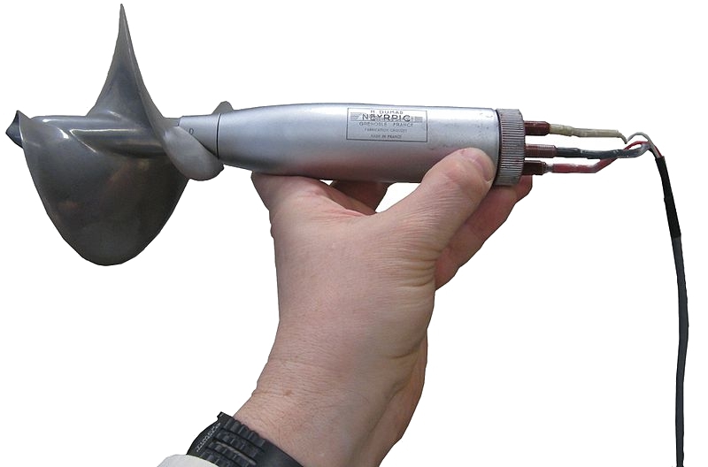
Instrumentos de medición
- Correntómetro de hélice (molinete): el instrumento clásico; la velocidad de rotación de la hélice es proporcional a la velocidad del agua.
- ADCP (Acoustic Doppler Current Profiler): mide el perfil completo de velocidades con ultrasonido; permite aforar desde una embarcación o sistema de teleférico en ríos grandes.
- Flotadores: método simple para caudales aproximados en emergencias; velocidad superficial × coeficiente de corrección.
Curva de gasto (rating curve)
Aforar un río en todas las crecidas es impracticable. Por eso se establece la curva de gasto, que relaciona el nivel (tirante) del río con el caudal. Una vez calibrada, basta con registrar el nivel de forma continua (con un limnígrafo o sensor de presión) para obtener el caudal correspondiente. Esta es la base de las estaciones hidrológicas de monitoreo.
Fuentes y lecturas recomendadas
- ISO 748:2007. Hydrometry — Measurement of liquid flow in open channels using current-meters or floats. ISO.
- WMO (2010). Manual on Stream Gauging. Vol. I: Fieldwork. WMO-No. 1044.
- Herschy, R. W. (2009). Streamflow Measurement. 3rd ed. Taylor & Francis.